R Programming

Quiz 1 Review

I will show the questions from quiz 1 that some students struggled with. Not including them in these slides in case I teach the course again in the future.

If you're arriving at this slide and are disappointed not to find quiz answers, I'm sorry but I'll at least give you this bit of entertainment. Go check out A Day in the Life of Americans

Intro to Functional Programming

R is a functional programming language. Functions enable you to write powerful, concise code.

"If you find yourself copying and pasting the same code more than twice, it's time to write a function." - Hadley Wickham

# Function to return only the numbers smaller than 10
nums <- c(1, 3, 4, 8, 13, 24)

getLittleNumbers <- function(some_numbahs){
    lil_ones <- some_numbahs[some_numbahs < 10]
    return(lil_ones)
}

getLittleNumbers(nums)

Positional and Keyword Arguments

When you call a function with arguments in R, you can provide those arguments two ways:

• "positional" = based on the order
• "keyword" = matching a specific argument by name

# all positional
rnorm(10, 0, 0.5)

# all keyword
rnorm(n = 10, mean = 0, sd = 0.5)

# mix
rnorm(10, mean = 0, sd = 0.5)

Required Arguments

• R functions take 0 or more arguments...basically named variables that the function uses to do it's work
• Take a look at ?sqrt. You'll see that it takes one argument, named x. You can pass any vector of numeric values to this argument and sqrt() will return the square root of each element
• In this case, we'd say x is a required argument of sqrt()

# Take the square root of a vector of numbers
sqrt(x = c(1, 4, 9, 16, 25))

# Note that calling this function without the argument will throw an error!
sqrt()
### Error in sqrt(): 0 arguments passed to `sqrt` which requires 1

Default Argument Values

• For more complicated functions, passing values to each argument can get burdensome
• To handle this, R allows function authors to specify default arguments. These are values that certain arguments will take automatically unless you decide to overwrite them
• Example: look at ?rnorm. You'll see that this function's signature reads rnorm(n, mean = 0, sd = 1).

# 100 random draws from a normal distribution w/ mean 0 and standard deviation 1
rand_nums <- rnorm(n = 100)

# 100 random draws from a normal distribution w/ mean 4.5 and standard deviation 1
rand_nums <- rnorm(n = 100, mean = 4.5)

Functions That Return Stuff

As you've seen in previous examples, the R special word return tells a function to "give back" some value When you execute an expression like x <- someFunction(), that function's return value (an R object) is stored in a variable called "x".

Unlike in some other programming languages, R allows you to use multiple return values inside the body of a function. The first time that the code inside the function reaches a return value, it will pass that value back out of the function and immediately stop executing the function.

See "Functions That Return Stuff" in the programming supplement.

Functions That Return Nothing

Not all functions have to return something! Sometimes you may want to create a function that just has some side effect like creating a plot, writing to a file, or print to the console.

These are called "null functions" and they're common in scripting languages like R. By default, these functions return the R special value NULL.

printSentence <- function(theSentence){
    words <- strsplit(x = theSentence, split = " ")
    for (word in words){
        print(word)
    }
}

# Assigning to an object is irrelevant...this function doesn't return anything
x <- printSentence("Hip means to know, it's a form of intelligence")
x

Scoping

Remember when we talked about namespaces and how R searches for objects? It's time to extend that logic to functions...which is where things get a bit weird and hard to understand.

R uses a search technique called lexical scoping

See "Scoping" in the programming supplement.

Looping with lapply()

R's *apply family of functions are a bit difficult to understand at first, but soon you'll come to love them. They make your code more expressive, flexible, and parallelizable (more on that final point later). One of the most popular is lapply() ("list apply"), which loops over a thing (e.g. vector, list) and returns a 1-level list. Let's try it out:

# Create a list
studentList <- list(
  wale = c(80, 90, 100)
  , talib = c(95, 85, 99)
  , common = c(100, 100, 99)
)

# Better way with lapply
grades <- lapply(studentList, mean)

Looping with sapply()

Remember that you cannot execute statistical operations like mean() over a list. For that, you'll want a vector of results. This is where R's sapply() ("simplified apply") comes in. sapply() works the same way that lapply() does but returns a vector. Try it for yourself:

data("ChickWeight")
weights <- ChickWeight$weight

# Loop over and encode "above mean" and "below mean"
the_mean <- mean(weights)
meanCheck <- function(val, ref_mean){
    if (val > ref_mean){return("above mean")}
    if (val < ref_mean){return("below mean")}
    return("equal to the mean")
}
check_vec <- sapply(weights, FUN = function(x){meanCheck(val = x, ref_mean = the_mean)})

Looping with apply()

When analyzing real-world datasets, you may want to use the same looping convention we've been discussing, but apply it over many items and the get some summary (such as the median) of the results. This is where R's apply() function comes in! Check it out:

data("ChickWeight")

# Calculate column-wise range
apply(ChickWeight, MARGIN = 2, FUN = function(x){range(as.numeric(x))})

# Calculate row-wise range
apply(ChickWeight, MARGIN = 1, FUN = function(blah){range(as.numeric(blah))})

Print Debugging

Writing code involves a never-ending process of trying this, fixing errors, trying other things, fixing new errors, etc. The process of identifying and fixing errors/bugs is called debugging.

The simplest way to debug an issue in your code is to use print debugging. This approach involves forming expectations about the state of the objects in your environment at each point in your code, then printing those states at each point to find where things broke.

See "Print Debugging" in the programming supplement for an example of this approach.

Googling Around

The second most popular debugging strategy:

Googling Around (continued)

But really...Google is your best friend. It will be particularly useful in the cases where your code is returning an error or warning. Simply pasting that output into a search engine (in quotes to get an exact match) will typically get you to an answer within 5 minutes.

Let's try an example.

Imagine that you got this error:

Error in sum(c(1, 2, "5")) : invalid 'type' (character) of argument.

Try to figure out what went wrong. HINT: it often helps to type the function name outside quotes. e.g. function "this is some error text"

Stack Overflow

You'll find yourself at https://stackoverflow.com/ OFTEN.

Building an MWE

If print debugging doesn't work, you may want to ask someone (a colleague, a package author, your teach) for help in debugging the issue. Before asking for someone's help, you owe it to them to try to reduce the problem to a Minimum Working Example (MWE), the simplest possible code that reproduces the error.

• this is bad
• this is good

In many instances, you'll find that just doing this exercise will reveal the problem before you even have to ask for anyone's help.

For more on building an MWE, see: "How to create a minimal, reproducible example" (link).

Built-in Docs with "?"

All R packages submitted to CRAN must supply some basic documentation for each function they contain. If a function is behaving strangely, it's often useful to look at the documentation under ?function_name.

For example, you may be surprised to learn that sum(c(1,2,NA,3)) evaluates to NA. You might have thought it would be 6. If we call ?sum in R, you'll see the answer...the default behavior of this function is to leave NA values in when calculating the sum, but there is an option argument na.rm that allows you to remove them if you wish.

Many IDEs (including RStudio) offer automatic code completion that will suggest these other arguments in the UI as you type!

Package Vignettes

What if you're not sure what functionality a package has? At least one source for this information is the package vignettes.

Let's take a look at the online documentation for the {stringr} package:

• CRAN docs: https://cran.r-project.org/web/packages/stringr/index.html
• package vignette: https://cran.r-project.org/web/packages/stringr/stringr.pdf

Looking at Source Code

If you try all the strategies we just discussed and STILL don't know why your code isn't working, try looking at the source code! Recall the following facts:

• R is open-source, which means that all R source code can be found online (typically on GitHub) and visually inspected
• Errors thrown by programs are not magical...they had to be written into the source code by a developer

For example, let's search for the error: each element of valids must have a name in the {lightgbm} source code. Please visit:

https://github.com/microsoft/LightGBM

Loading Installed Packages

As you advance in R, you will find that the functions provided by packages like {base}, {stats}, and {utils} are not sufficient. For example, you may want to use {dygraphs} to make interactive plots.

# Load dependencies
library(data.table); library(dygraphs); library(quantmod);

# Get data
cpiData <- quantmod::getSymbols(
    Symbols = "CPIAUCSL", src = "FRED", auto.assign = FALSE
)["1947-01-01/2023-11-01"]

# Plot it
dygraphs::dygraph(
    data = cpiData, main = "U.S. CPI", xlab = "date", ylab = "Index (1982-1984 = 100)", elementId = "plot"
) %>%
    dygraphs::dyRangeSelector()

Installing from CRAN

CRAN, "The Comprehensive R Archive Network", is the main server from which you'll download external packages. It provides an easy framework for distributing code (way better than passing around hundreds of links to GitHub repos).

To download and install packages, do the following:

# Install packages + their dependencies with install.packages()
install.packages(c("data.table", "jsonlite"),
                 dependencies = c("Depends", "Imports"))

# Load package namespace with library()
library(data.table)

# (A few months later...) Check CRAN for new versions of your packages
utils::update.packages()

Installing from GitHub

While there are many many packages available from CRAN, you may sometimes want to install directly from a source control site like GitHub. R developers will often release bleeding-edge ("dev") features on GitHub before they make it to CRAN.

# Load deps
library(remotes)

# Install from GitHub
remotes::install_github("terrytangyuan/dml")

# Check where R put this package on your machine
find.package("dml")

Namespacing Calls

You may have noticed that I use :: frequently in my code. Remember when we used search() to print the ordered list of namespaces that R searches for objects? :: is used to circumvent this process. lubridate::ymd_hms() tells R "Use the function ymd_hms from the 'lubridate' package"

Without namespacing, R will search through the list of namespaces until it finds what it wants. When you load a new package that has a function with the same name as one already loaded in your session, R will warn you that that version has been "masked".

library(lubridate)

Attaching package: 'lubridate'

The following object is masked from 'package:base':

    date

library() vs. require()

In this course, I've been using the library() command to load package namespaces. If you look around online, you will probably see many examples where people use require() instead.

what's the difference?

• library() is used in scripts. It will throw an error if you do not have the package
• require() is used in functions. It will throw a warning if you don't have the package
• Errors will break your code immediately, while warnings will print a note but allow the code to keep running

library(some_package_that_does_not_exist)

my_func <- function(n){
    require(some_package_that_does_not_exist)
    print("JaVale McGee!!!!")
}

Using Local Code with source()

For your own reusable code, you may find it convenient to define functions in a separate file and use source() to make those functions available to other scripts.

my_script.R

# load function
source("helper_functions.R")

myData <- createRandomData(100, "norm")

head(myData)

See "Sourcing Helper Functions" in the programming supplement for an example.

File Paths

Whenever you find yourself reading data into R or writing data out of it, you will need to work with file paths. File paths are just addresses on your computer's file system. These paths can either be relative (expressed as steps above/below your current location) or absolute (full addresses).

All relative paths in R are relative to your working directory, a single location that you can set and reset any time in your session.

relative path: "file.txt"

absolute path: "/Users/jlamb/repos/some-project/data/file.txt"

See "File Paths" in the programming supplement.

File Paths

R provides a few other utilities for working with file paths and directory structures.

• getwd(): print the current working directory
• list.files(): get a character vector with names of all files found in a directory
• file.path(): create a filepath from multiple parts
• file.exists(): returns TRUE is a file exists and FALSE if it doesn't
• dir.exists(): returns TRUE is a directory exists and FALSE if it doesn't
• dir.create(): create a new directory

See "File Paths" in the programming supplement.

Downloading files from the internet

To download files hosted on the internet, you can use download.file().

iris_url <- paste(
    "https://raw.githubusercontent.com/jameslamb/intro-to-r/main/sample-data/iris.csv"
    , collapse = "/"
)

download.file(
  url = iris_url
  , destfile = "iris.csv"
)

Delimited Files

Out in the wild, one of the most common types of flat file you will find is a delimited file. In these files, bits of data are separated by a common character ("delimiter"). Common types include comma separated values (CSV), tab-separated values, and space-delimited. When these files are opened by a program like R, SAS, or Excel, those programs can figure out what the delimiter is and use it to split data into columns.

CSV

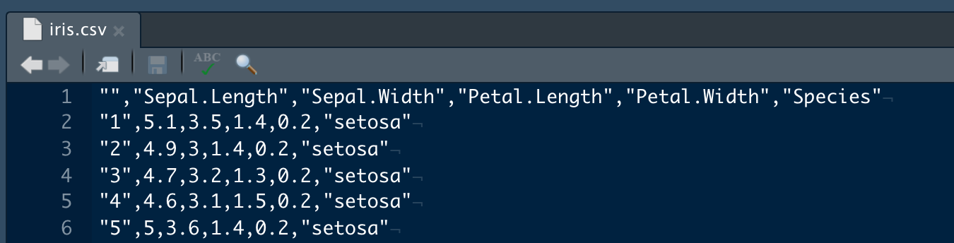
CSV ("comma-separated values") is a really common format to share small datasets because it is just a text file, and can be ready by many different types of programs. R has several options for reading this type of file.

• read.csv(): base R function for reading CSVs into a data.frame
• read.delim(): similar to read.csv(), but can read files with any delimiter
• arrow::read_csv_arrow(): fast CSV reader using a high-performance data frame library called Apache Arrow
• data.table::fread(): super-fast CSV reader that creates a special type of data.frame called a data.table
• readr::read_csv(): CSV reader from RStudio

See "CSV" in the programming supplement for an example of working with CSVs.

Excel

Many organizations share data in Microsoft Excel workbooks.

There are a few packages for reading and writing Excel files in R.

• {openxlsx}
• {readxl}
• {xlsx}

See "Excel" in the programming supplement for an example with {openxlsx}.

JSON

JSON ("Javascript Object Notation") is a standard format for "semi-structured" or "nested" data. It's a plain-text format that can be used by many programs and programming languages.

{
  "status": 200,
  "data": [
    {"customer_name": "Lupe", "purchases": 10},
    {"customer_name": "Wale", "purchases": 30}
  ]
}

This type of data is commonly represented as an R list. See "JSON" in the programming supplement for an example using some JSON data from the GitHub API.

Unstructured Text Files

Text files that are "unstructured" don't cleanly map to an R data structure like a data frame, matrix, or list. An example might be a collection of court transcripts.

The best we can do with these is read them into character vectors, where each element in the vector corresponds to one line in the file.

See "Unstructured Text Files" in the programming supplement for some hands-on experience with this approach.

Learning More on Your Own

See the links below to learn more about some of the topics we covered this week

Debugging R code: RStudio debug mode | R-bloggers | Stack Overflow

External R Packages: econometrics packages | finance packages | time series packages

Lexical Scoping: "R Programming for Data Science" book