R Programming
Week 1
Contents
Introduction
- Introduction 6
- Syllabus Review 7
- Course Objectives 8
Setting Up Your Environment
- Installing R + RStudio 10
- Authoring Scripts in RStudio 11
- Authoring Scripts in a Text Editor 12
- Executing R Code 13-14
Introduction to R
- R is an interpreted language 16
- R is dynamically typed language 17
- R has a few of its own file types 18
Programming Fundamentals
- Variables and Namespaces 20
- Introduction to Types 21
- Dollarstore Calculator Math 22-24
Contents
R Data Structures
- Vectors 26-27
- Lists 28
- Factors 29
- Data Frames 30
Logical Operators
- Logical Operators 32-34
Subsetting
- Subsetting Vectors 36
- Subsetting Lists 37
- Subsetting Data Frames 38
- Using Logical Vectors 39
Controlling Program Flow
- If-Else 40-42
- For Loops 43
- While Loops 44
Additional Resources
- Learning More on Your Own 46
Introduction
Personal Introduction
My Marquette Experience:
- B.S., Economics & Marketing (2013), M.S.A.E. (2014)
Since Marquette:
- Software Engineer @ NVIDIA, 2023-present
- Data Scientist/Engineer @ Uptake, AWS, Saturn Cloud, SpotHero 2016-2023
- M.I. in Data Science, University of California - Berkeley (MIDS)
- Co-author and maintainer of
{uptasticsearch}and{pkgnet}packages on CRAN - Maintainer on
LightGBM - Created "Timeseries with data.table in R" DataCamp course
- Analyst/Economist @ IHS Economics, Abbott Laboratories, 2014-2015
Syllabus review

Course Objectives
The main objectives for the course are as follows:
- Set up a data science software stack on your machine
- Learn how to author and manage a statistical code base
- Learn the basics of manipulating data using R
- Learn how to incorporate external packages to make your scripts more powerful
- Practice solving problems in R and presenting solutions in a code review format
Setting Up Your Environment
Installing R + RStudio
Programming in R begins with installing R!
- Go to https://cran.r-project.org/
- Choose the appropriate download for your operating system (you'll see links like "Download R for Mac OS")
- Open the file and follow the prompts on the screen
R comes with a command-line client and a default GUI, but most users prefer to use other IDEs ("integrated development environment"). The most popular IDE for R, and the one we'll use in this class, is RStudio:
- Go to https://posit.co/products/open-source/rstudio/
- Choose the appropriate download under "All Installers"
- Open the file and follow the prompts on the screen
Authoring Scripts in RStudio
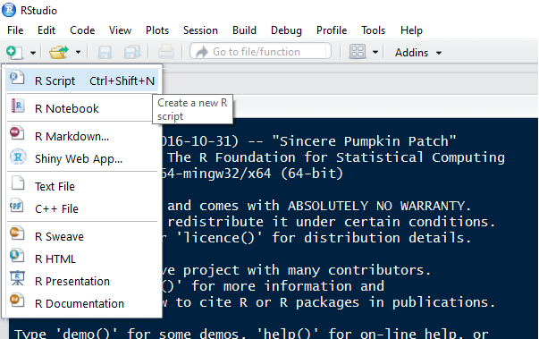
Sequences of R code are typically saved in scripts with the file extension ".R". To open a blank script in RStudio and start editing, you can either go to "File --> New File --> R script" or choose "R Script" from the paper image in RStudio:
Authoring Scripts in a Text Editor
When you author a script in RStudio, the file you create will be stored with the file extension ".R" by default. Out in the wild (i.e. editing in text editors), you are responsible for saving files with the appropriate file extension so the software that uses them can interpret them correctly. Trust me, there are a lot of them
A few common ones you'll want to know for this course:
Scripts and Docs
- General text files (.md, .txt)
- R scripts (.R, .r)
- SQL queries (.sql)
- Slides and reports (.css, .html, .pdf, .rmd)
Data
- API response data (.csv, .json, .xml)
- R data formats (.rda, .rds, .RData)
- MS Excel (.xls, .xlsx, .xlsm)
- Zip archives (.zip, .tar, .gz, .bzip2)
Executing R Code: RStudio
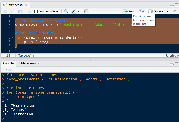
R is an interpreted language (more on this later). TL;DR, you need to send your code to some software that knows what to do with it ("R"). RStudio makes this super easy to do. You can execute your code interactively (one line at a time) in the R console or run your .R scripts using the "run" button.
Using Scripts
The Console
Executing R Code: The Command Line
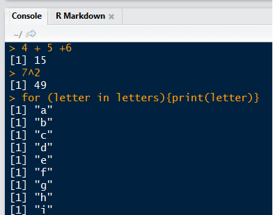
When R is just one of the tools in your stack, it's often quicker to execute your code from a terminal rather than going into a dedicated application for each type of file.
The R REPL
- R comes with a REPL (read-eval-print loop) which allows you to quickly turn a terminal command line into an R console.
- To activate:
Rfrom the command line - To close:
quit()orq()
Rscript
- If your commands are stored in a ".R" script, you can execute that script from the command line with the
Rscriptcommand. - This command will run all the lines in the file in the order they've been written and potentially output some messages to the terminal.
Introduction to R
R is an Interpreted Language
Interpreted languages are those which break commands down into building blocks called "subroutines" that have already been compiled in machine code (source: Wikipedia). Much of the R source code (including these subroutines) is actually written in C.
To ensure that that process of breaking down ("interpreting") code goes smoothly, R needs to use a few keywords to identify crucial operations. Like other scripting languages, it has a set of "reserved words" which you cannot use as object names.
Run ?reserved in RStudio
Run TRUE = 4 in RStudio
R is a Dynamically Typed Language
Some languages like Java required you to declare the types of objects you create
- for example: string, numeric, integer, or boolean
- pros: strong typing makes software faster and more reliable (broadly speaking)
- cons: code is very verbose, difficult to prototype in and debug
R is "dynamically typed"
- this means that you can create objects without explicitly telling R "this is an integer"
- in addition, you're free to re-assign variable names to different types at any time in scripts
R has its own File Types
| Extension | Description |
|---|---|
| .r, .R | Text format for scripts. |
| .rda, .RData | R data format. One or many R objects |
| .rds | R data format. Single R object. Can be loaded into a named object |
# .r and .R scripts can be run inside R with source()
source("my_script.R")

# .rda and .RData files can be loaded into an R session with load()
load("all_of_the_data.rda")

# .rds files can be read directly into an R object
someData <- readRDS("my_data.rds")
Programming Fundamentals
Variables and Namespaces
When you execute a statement like x <- 5 in R, you are creating an object in memory which holds the numeric value 5 and is referenced by the variable name "x".
If you later ask R to do something like y <- x + 2, it will search through a series of namespaces until it finds a variable called "x". Namespaces can be thought of as collections of labels pointing to places in memory. You can use R's search() command to examine the ordered list of namespaces that R will search in for variables.
# Check the search path of namespaces
search()

# use ls() to list the objects in one of those namespaces
ls("package:stats")
Introduction to Types
Languages like Java and C are more verbose than R partially because they require programmers to explicitly declare types for data values. We will not go into the intricacy of typing in this course, but you should be familiar with the following types (this knowledge will serve you well across all languages):
- integer: non-complex whole numbers. created with an L like
anInteger <- 1L - numeric: all real numbers. Default type for numbers in R
someNums <- c(1.005, 2) - logical: TRUE or FALSE.
someLogicals <- c(TRUE, FALSE, FALSE) - character: strings of arbitrary characters. Sometimes referred to informally as "text data".
stringVar <- "Chicago Heights"
Dollarstore Calculator Math (pt 1)
# Addition with "+"
4 + 5
## [1] 9
# Subtraction with "-"
100 - 99
## [1] 1
Dollarstore Calculator Math (pt 2)
# Multiplication with "*"
4 * 5
## [1] 20
# Division with "/"
15 / 3
## [1] 5
# Exponentiation with "^"
2^3
## [1] 8
Dollarstore Calculator Math (pt 3)
# Order of Operations
4 * 5 + 5 / 5
## [1] 21
# Control with parentheses
4 * (5 + 5) / 5
## [1] 8
Data Structures
Vectors (pt 1)
- Because R was designed for use with statistics, most of its operations are vectorized
- You can create vectors a few ways:
# Ordered sequence of integers
1:5

# Counting by 2s
seq(from = 0, to = 14, by = 2)

# Replicate the same values
rep(TRUE, 6)

# Concatenate multiple values with the "c" operator
c("all", "of", "the", "lights")
Vectors (pt 2)
- Vectors are at the heart of many R operations. Try a few more practice exercises:
# Watch out! Mixing types will lead to silent coercion
c(1, TRUE, "hellos")

# Some functions, when applied over a vector, return a single value
is.numeric(rnorm(100))

# Others will return a vector of results
is.na(c(1, 5, 10, NA, 8))

# Vectors can be named
batting_avg <- c(youkilis = 0.300, ortiz = 0.355, nixon = 0.285)

# You can combine two vectors with c()
x <- c("a", "b", "c")
y <- c("1", "2", "3")
c(x, y)
Lists
Vectors are the first multi-item data structure all R programmers learn. Soon, though, you may find yourself frustrated with the fact that they can only hold a single type. To handle cases where you want to package multiple types (and even multiple objects!) together, we will turn to a data structure called a list.
| Capabilities | Vectors | Lists |
|---|---|---|
| Optional use of named elements | ✔ | ✔ |
| Support math operations like mean() | ✔ | |
| Hold multiple types | ✔ | |
| Hold multiple objects | ✔ |
# Create a list with list()
myList <- list(a = 1, b = rep(TRUE, 10), x = c("shakezoola", "mic", "rulah"))

# Examine it with str()
str(myList)
Factors
R comes with a special type called a "factor" for modelling categorical variables. To save memory, internally R will convert factor values to integers and then keep around a single table that says, for example, 1 = "Africa", 2 = "Asia", etc.
regions <- as.factor(c("Africa", "Asia", "Europe", "Asia"))
region_fac <- as.factor(regions)
print(region_fac)
## [1] Africa Asia   Europe Asia
## Levels: Africa Asia Europe
print(as.integer(region_fac))
## [1] 1 2 3 2
See "Factors" in the programming supplement for an example.
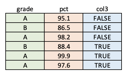
Data Frames
Data frames are tables of data. Each column of a data frame can be a different type, but all values within a column must be the same type.
See "Data Frames" in the programming supplement for some examples.
Logical Operators
Logical Operators
Often in your code, you'll want to do/not do something or select / not select some data based on a logical condition (a statement that evaluates to TRUE or FALSE).
# "and" logic is expressed with "&"
TRUE & TRUE   # TRUE
TRUE & FALSE  # FALSE
FALSE & FALSE # FALSE
-5 < 5 & 3 > 2 # TRUE

# "or" logic is expressed with "|"
TRUE | TRUE    # TRUE
TRUE | FALSE   # TRUE
FALSE | FALSE  # FALSE
3 < 8 | 8 > 19 # TRUE
Logical Operators (continued)
The most common operators used to generate logicals are >, <, ==, and !=
# "equality" logic is specified with "=="
3 == 3   # TRUE
4 == 4.1 # FALSE

# "not" logic is specified with !. In a special case, != signifies "not equal"
!TRUE            # FALSE
!FALSE           # TRUE
! (TRUE | FALSE) # FALSE
4 != 5           # TRUE

# "greater than" and "less than" logic are specified in the way you might expect
5 < 5  # FALSE
6 <= 6 # TRUE
4 > 2  # TRUE
3 >= 3 # TRUE
Logical Operators (continued)
As a general rule, when you put a vector on the left-hand side of a logical condition like == or >, you will get back a vector as a result.
vehicleSizes <- c(1, 5, 5, 2, 4)

# Create a logical index. Note that we get a VECTOR of logicals back
bigCarIndex <- vehicleSizes > 4

# Taking the SUM of a logical vector tells you the number of TRUEs.
sum(bigCarIndex)

# Taking the MEAN of a logical vector tells you the proportion of TRUEs
mean(bigCarIndex)
Subsetting
Subsetting Vectors
Subsetting is the act of retrieving a portion of an object, usually based on some logical condition (e.g. "all elements greater than 5"). In R, this is done with the [ operator.
# Create a vector to work with
myVec <- c(var1 = 10, var2 = 15, var3 = 20, av4 = 6)

# "the first element"
myVec[1]
## var1
##   10
# "second to fourth elements"
myVec[2:4]
## var2 var3  av4
##   15   20    6
# "the element named var3"
myVec["var3"]
## var3
##   20
Subsetting Lists
Lists, arbitrary collections of R objects, support three subsetting operators.
[= returns a 1-element listsomeList["grades"]someList[1]
[[= returns the object in its natural form (whatever it would look like if it wasn't in a list)someList[["grades"]]someList[[1]]
$= similar to[[, but uses unquoted keys and cannot use positionssomeList$grades
Please see "Subsetting Lists" in the programming supplement.
Subsetting Data Frames
Data frames are the workhorse data structure of statistics in R. The best way to learn data frame subsetting is to just walk through the examples below:
# Create a data frame
someDF <- data.frame(
    , conference  = c("Big East", "Big Ten", "Big East", "ACC", "SEC")
    , school_name = c("Villanova", "Minnesota", "Marquette", "Duke", "LSU")
    , wins        = c(18, 14, 19, 24, 12)
    , ppg         = c(71.5, 45.8, 66.9, 83.4, 58.7)
)

# Grab the wins column (NOTE: will give you back a vector)
someDF[, "wins"]

# Grab the first 3 rows and the two numeric columns
someDF[1:3, c("wins", "ppg")]
Using Logical Vectors
So far, we've seen how to subset R objects using numeric indices and named elements. These are useful approaches, but both require you to know something about the contents of the object you're working with.
Using these methods (especially numeric indices like saying give me columns 2-4) can make your code confusing and hard for others to reason about. Wherever possible, I strongly recommend using logical vectors for subsetting. This makes your code intuitive and more flexible to change.
Please see "Using Logical Vectors" in the programming supplement for an example.
Controlling Program Flow
Controlling Program Flow: If-Else
Soon after you start writing code (in any language), you'll find yourself saying "I only want to do this thing if certain conditions are met". This type of logic is expressed using if-else syntax)
x <- 4
if (x > 5){
    print("x is above the threshold")
}
See "If-Else" in the programming supplement for more examples.
If-Else (continued)
What if you want to express more than two possible outcomes? For this, we could use R's else if construct to nest conditions. Note that conditional blocks can have any number of "else if" statements, but only one "else" block.
# Try to think through what this will do before you run it yourself
if (4 > 5){
    print("3")
} else if (6 <= (5/10)) {
    print("1")
} else if (4 + 4 + 4 == 12.0001) {
    print("4")
} else {
    print("2")
}
For Loops
One of the most powerful characteristics of general purpose programming languages is their ability to automate repetitive tasks. When you know that you want to do something a fixed number of times (say, squaring each item in a vector), you can use a for loop.
# Create a vector
x <- c(1, 4, 6)

# Print the square of each element one at a time
print(1^2)
print(4^2)
print(6^2)

# BETTER: Loop over the vector and print the square of each element
for (some_number in x){
    print(some_number^2)
}
While Loops
For loops are suitable for many applications, but they can be too restrictive in some cases. When you want to say "run this code until some condition is met", a while loops is more appropriate.
i <- 1
while (i < 5) {
    print(i)
    i <- i + 1
}
## [1] 1
## [1] 2
## [1] 3
## [1] 4
See "While Loops" in the programming supplement for a hands-on example.
Additional Resources
Learning More on Your Own
For the brave and curious, I've included a few online free resources for learning more about the technologies we discussed.
R: swirl | JHU Data Science
RStudio: RStudio blog
Subsetting: Quick-R | R-bloggers | Advanced R book